Limitations in usefulness of conventional standard deviation bands as overbought/oversold benchmarks
One of the popular ways of detecting a trend in financial market time series corrupted by random fluctuations (noise) is moving average smoothing. Actual prices fluctuate around the moving average. To measure an average distance of price values from the moving average the standard deviation (SD) can be used. The so-called in statistics "range rule of thumb" determines the range of price variability around the moving average as approximately 4SD, providing confidence limit of about 95.5 %. According to the rule, the upper boundary of the range will be about 2SD above the moving average and the lower boundary of the range will be about 2SD below the moving average. In order to get higher confidence of the projected range, its half-bandwidth should be widened, for example to 3SD. The probability that the price data will be within plus or minus three standard deviations from moving average is equal in this case to 99.7%. As you can see from above, the primary function of the conventional standard deviation bands is to estimate the range of price variability around the moving average and indicate the current disposition of the price in relation to the moving average and the bands. The commonly used for this purpose 2SD bands are known in technical analysis as Bollinger Bands. Mr. Bollinger recommends using a 20-point period simple moving average of typical price for their calculation.
Can Bollinger Bands be used as overbought/oversold benchmarks? Some traders believe that Bollinger Bands offer an effective tool for indicating overbought/oversold conditions and oncoming reversals in a trend. And many traders criticize them for not providing more straightforward readings of price extremes. The thing is that when price is losing momentum it deviates from the bands in advance, much before it reaches the extremities. That is why when prices hit the upper or lower boundaries of the bands this it is not necessarily an indication of their extremes. It just means that prices have reached the limits of the established range. That's why traders would have to use other indicators in conjunction with these price bands to determine the overbought/oversold conditions and the reversal points of the trend. The same limitation refers to the derivative indicators, such as the "%b" indicator, and CCT Bollinger Bands Oscillator provided by Steve Karnish.
In this article, we will show how to make standard deviation bands adequately fulfill a function of providing overbought/oversold benchmarks.
Quantitative criterion of functioning
To trade successfully the benchmarks of overbought/oversold indicators must be set so that most of valid signals could penetrate them providing a reliable indication of the security's overbought/oversold conditions. Our study of the problem shows that about 60% of all signals generated by any trading rule, for example by price and moving average crossover rule, must penetrate overbought/oversold benchmarks, and 40 % of the signals, which are supposed be false reversals typical for congestion and transition phases, must be rejected. For ranging and weakly trending markets (Dow retracement > 0.5) about 20% to 30% of the points falling outside the benchmarks meet this criterion, providing reliable readings of a security's overbought/oversold conditions. This proportion must therefore be attributed to the standard deviation bands to turn them into the overbought/oversold benchmarks. It was found that the required proportion is provided by the half-bandwidth of the bands equal to 1.4 SD. That is, the upper boundary of the bands will be about 1.4 SD above the moving average, and the lower boundary of the bands will be about 1.4 SD below the moving average.
Dual representation of the indicator
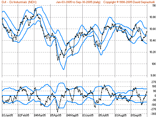
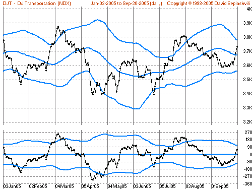
The 1.4-standard deviation price bands as overbought/oversold indicator can be easily reconfigured into an oscillator format. The indicator in this format consists of the conventional price oscillator calculated as difference between price and its moving average, and 1.4 SD overbought and oversold boundaries plotted above and below zero line. The oscillator fluctuates around the zero line and inside and outside the 1.4 SD boundaries. Penetration of the upper boundary indicates overbought conditions, while penetration of the lower boundary signifies oversold conditions. By way of illustration see in Figure 1 of DJ Industrial Index the 10-day period indicator, and in Figure 2 of DJ Transportation Index the 40-day period indicator, both in price chart and oscillator formats. The offered oscillator determines not only overbought/oversold conditions but also defines volatility. You can see how harmonically the overbought/oversold bands contract during less volatile periods, and how the bands expand during more volatile periods. Low readings of volatility, typically preceding a large move in the security's price, clearly indicate congestion and transition zones, which better be skipped.
If you draw a parallel between the price chart and the price oscillator configurations of the indicator, you will see that they serve one and the same purpose in different formats. The difference is not functional, but representational and you can choose to use the format of your preference.
Empirical confirmation
Let's see how the indicator fits the criterion of functioning. Market indexes are probably most useful for verification, as three out of four securities, as a rule, follow them. Below, in Table 1, testing results of the offered overbought/oversold indicator on DJ Industrial, S&P 500, and Nasdaq indexes are presented.
Table 1. Percentage of points falling outside the range of overbought-oversold levels
All of the most popular technical analysis indicators are explicitly or implicitly based on the assumption that price time series can be presented sufficiently well with one dominant cycle, which reflects the main dynamic properties of a security in the given time span. It is believed that the period of the indicator, approximately equal to half the period of the expected dominant time cycle, will be appropriate to extract actual cycles with this and higher periods, for example, the 10-day period indicator will reveal cycles of a 20-day and higher length in time series data. It is clear that the indicator will be successful as much as this predetermined period fits actual price movement. However, it should be admitted without going into detail, that there are no magic, consistent periods in price non-periodic noisy time series, and a trader who believes cries for the moon. The lack of efficiency of such generalization can be compensated by occasional control and retuning of the indicator's period, or by using a multi-frame indicator. In either case it is required that indicator be able to operate over different time periods. As you can see from the table, the offered indicator meets both formulated requirements: the percentage of points falling outside the overbought-oversold range of all tested indexes are confined to an acceptable interval of values and the indicator performs equally well in all used in trading practice calculation periods. Testing results on a wide diversity stocks, index shares, and indexes in various market conditions confirm these results and show that the offered indicator can ensure clear
signaling of overbought-oversold conditions.
How informative overbought/oversold benchmarks are with momentum indicators and the ways to make them adaptive to the markets they are measuring you can find in my article published in November 2005 issue of the Futures magazine.
One of the popular ways of detecting a trend in financial market time series corrupted by random fluctuations (noise) is moving average smoothing. Actual prices fluctuate around the moving average. To measure an average distance of price values from the moving average the standard deviation (SD) can be used. The so-called in statistics "range rule of thumb" determines the range of price variability around the moving average as approximately 4SD, providing confidence limit of about 95.5 %. According to the rule, the upper boundary of the range will be about 2SD above the moving average and the lower boundary of the range will be about 2SD below the moving average. In order to get higher confidence of the projected range, its half-bandwidth should be widened, for example to 3SD. The probability that the price data will be within plus or minus three standard deviations from moving average is equal in this case to 99.7%. As you can see from above, the primary function of the conventional standard deviation bands is to estimate the range of price variability around the moving average and indicate the current disposition of the price in relation to the moving average and the bands. The commonly used for this purpose 2SD bands are known in technical analysis as Bollinger Bands. Mr. Bollinger recommends using a 20-point period simple moving average of typical price for their calculation.
Can Bollinger Bands be used as overbought/oversold benchmarks? Some traders believe that Bollinger Bands offer an effective tool for indicating overbought/oversold conditions and oncoming reversals in a trend. And many traders criticize them for not providing more straightforward readings of price extremes. The thing is that when price is losing momentum it deviates from the bands in advance, much before it reaches the extremities. That is why when prices hit the upper or lower boundaries of the bands this it is not necessarily an indication of their extremes. It just means that prices have reached the limits of the established range. That's why traders would have to use other indicators in conjunction with these price bands to determine the overbought/oversold conditions and the reversal points of the trend. The same limitation refers to the derivative indicators, such as the "%b" indicator, and CCT Bollinger Bands Oscillator provided by Steve Karnish.
In this article, we will show how to make standard deviation bands adequately fulfill a function of providing overbought/oversold benchmarks.
Quantitative criterion of functioning
To trade successfully the benchmarks of overbought/oversold indicators must be set so that most of valid signals could penetrate them providing a reliable indication of the security's overbought/oversold conditions. Our study of the problem shows that about 60% of all signals generated by any trading rule, for example by price and moving average crossover rule, must penetrate overbought/oversold benchmarks, and 40 % of the signals, which are supposed be false reversals typical for congestion and transition phases, must be rejected. For ranging and weakly trending markets (Dow retracement > 0.5) about 20% to 30% of the points falling outside the benchmarks meet this criterion, providing reliable readings of a security's overbought/oversold conditions. This proportion must therefore be attributed to the standard deviation bands to turn them into the overbought/oversold benchmarks. It was found that the required proportion is provided by the half-bandwidth of the bands equal to 1.4 SD. That is, the upper boundary of the bands will be about 1.4 SD above the moving average, and the lower boundary of the bands will be about 1.4 SD below the moving average.
Dual representation of the indicator
The 1.4-standard deviation price bands as overbought/oversold indicator can be easily reconfigured into an oscillator format. The indicator in this format consists of the conventional price oscillator calculated as difference between price and its moving average, and 1.4 SD overbought and oversold boundaries plotted above and below zero line. The oscillator fluctuates around the zero line and inside and outside the 1.4 SD boundaries. Penetration of the upper boundary indicates overbought conditions, while penetration of the lower boundary signifies oversold conditions. By way of illustration see in Figure 1 of DJ Industrial Index the 10-day period indicator, and in Figure 2 of DJ Transportation Index the 40-day period indicator, both in price chart and oscillator formats. The offered oscillator determines not only overbought/oversold conditions but also defines volatility. You can see how harmonically the overbought/oversold bands contract during less volatile periods, and how the bands expand during more volatile periods. Low readings of volatility, typically preceding a large move in the security's price, clearly indicate congestion and transition zones, which better be skipped.
If you draw a parallel between the price chart and the price oscillator configurations of the indicator, you will see that they serve one and the same purpose in different formats. The difference is not functional, but representational and you can choose to use the format of your preference.
Empirical confirmation
Let's see how the indicator fits the criterion of functioning. Market indexes are probably most useful for verification, as three out of four securities, as a rule, follow them. Below, in Table 1, testing results of the offered overbought/oversold indicator on DJ Industrial, S&P 500, and Nasdaq indexes are presented.
Table 1. Percentage of points falling outside the range of overbought-oversold levels
| ||||||||||||||||||||||||||||||||||||||||
|
All of the most popular technical analysis indicators are explicitly or implicitly based on the assumption that price time series can be presented sufficiently well with one dominant cycle, which reflects the main dynamic properties of a security in the given time span. It is believed that the period of the indicator, approximately equal to half the period of the expected dominant time cycle, will be appropriate to extract actual cycles with this and higher periods, for example, the 10-day period indicator will reveal cycles of a 20-day and higher length in time series data. It is clear that the indicator will be successful as much as this predetermined period fits actual price movement. However, it should be admitted without going into detail, that there are no magic, consistent periods in price non-periodic noisy time series, and a trader who believes cries for the moon. The lack of efficiency of such generalization can be compensated by occasional control and retuning of the indicator's period, or by using a multi-frame indicator. In either case it is required that indicator be able to operate over different time periods. As you can see from the table, the offered indicator meets both formulated requirements: the percentage of points falling outside the overbought-oversold range of all tested indexes are confined to an acceptable interval of values and the indicator performs equally well in all used in trading practice calculation periods. Testing results on a wide diversity stocks, index shares, and indexes in various market conditions confirm these results and show that the offered indicator can ensure clear
signaling of overbought-oversold conditions.
How informative overbought/oversold benchmarks are with momentum indicators and the ways to make them adaptive to the markets they are measuring you can find in my article published in November 2005 issue of the Futures magazine.
Last edited by a moderator: