Bollinger Bands are among the most commonly found technical indicators these days. Even the most basic of charting applications include them among the available offerings. There are many ways the Bands can be incorporated in to one's market analysis and trading methods (see Bollinger Bands - The Basic Rules for a discussion). This article focuses on how they can be used to find markets in the early stages of significant directional moves.
The process of trend identification using Bollinger Bands starts with evaluating the width of the Bands. This is done using the Band Width Indicator (BWI), which is calculated as follows:
BWI = ( UB - LB ) / MB
Where UB is the Upper Band, LB is the Lower Band, and MB is the Middle Band.
Using the common default setting of 20-periods, that means the MB is the 20-period moving average. That default will be the one used in the examples provided herein, though it is by no means necessarily the best option.
The formula above will express the width between the Bands as a percentage of the moving average being used. It could be multiplied through by 100 to provide an integer value (as done on the sample charts). The average (MB) is used rather than current price because it is the central point in the Bands, whereas price could be anywhere within (or even outside) them.
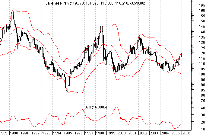
The reason for calculating BWI is that it gives us a normalized reading of how wide the Bands are for comparative purposes. A 100 point band width on the S&P 500, for example, is relatively different when the index is at 900 than when it's at 1500. The chart below provides an example of BWI. It is a daily chart of USD/JPY with the Bollinger Bands plotted along with price in the upper portion and BWI as the secondary plot below.
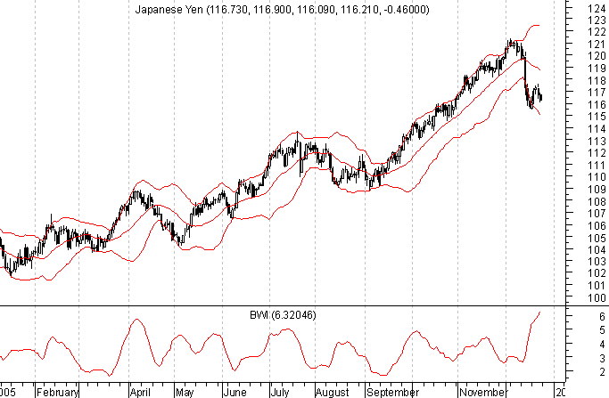
As you can see, BWI ranged between a bit below 2% and about 7% over the course of 2005. It is the lower extremes in the indicator readings which are the focus when one uses Bollinger Bands to help identify pending trends.
Continuing with USD/JPY, we can see a fairly recent example of what we are looking for here. Notice in the chart which follows, how narrow the Bollinger Bands became in September. According to BWI, they got to a width of less than 2%. Shortly thereafter, the market took off on a three month rally.
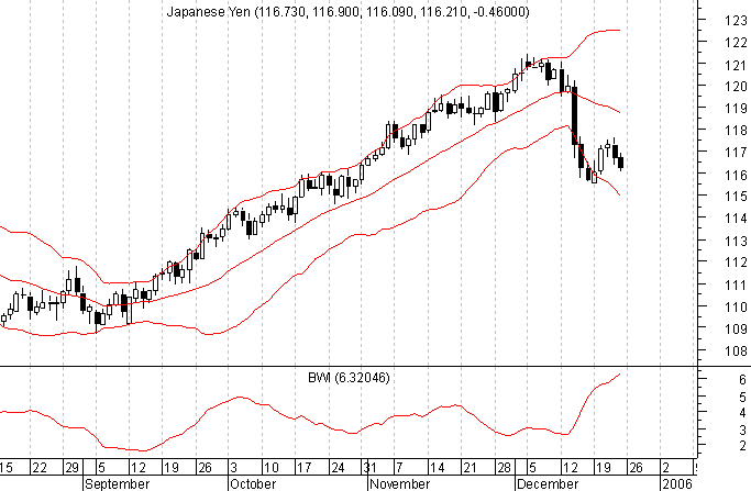
You can see from the following chart that the low BWI reading in September matched one from earlier in the year before a nice upswing in USD/JPY. It was also close to where the indicator got prior to the fall in the market late in 2004.
In the examples above, the bottom end of the BWI range was 1%-2%. For USD/JPY and some other markets such as the S&P, on a daily basis, readings that low are significant. In other markets, however, the scale is different. Look at Crude Oil, for example.
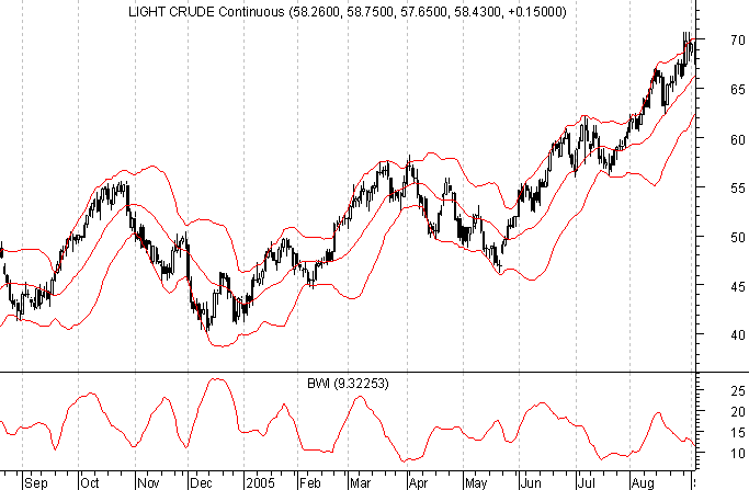
During the 12 months between August 2004 and August 2005, the lower bound was closer to 10%. That is reflective of how much more volatile Crude Oil prices were in that span than was true for other markets.
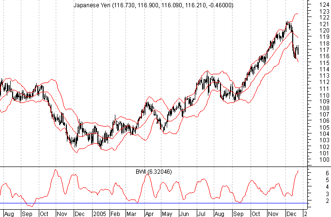
There are also differences in timeframe. Take a look at the monthly USD/JPY chart below to see how this can be the case.
Notice that BWI bottomed out around 10%, significantly above the 2% area seen on the daily chart. This, of course, is to be expected given the larger price moves which take place in that timeframe. The point, though, is that the process remains the same - look for a market situation in which BWI has reached a relatively low level in historic comparison, regardless of the timeframe in question.
What you are identifying when finding low BWI readings is markets which have been relatively range-bound for a period of time. The tendency is that the longer a market remains narrowly traded (low BWI), the more significant and explosive the move which follows. Some markets make these moves in fairly orderly fashions, as the USD/JPY example earlier. That was a fairly gradual, though quite sustained trend which began from a low BWI reading.
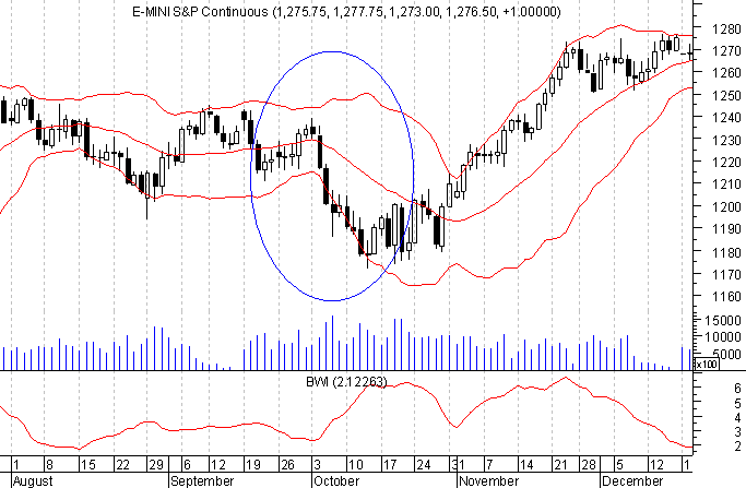
Other situations are more explosive. Take a look at the circled area on the S&P chart below (continuous contract E-minis). The BWI reading reached about 2%, which is pretty low for the index on the daily timeframe. The move which followed dropped the market 40-50 points in less than two weeks.
When reviewing BWI, it is generally not enough to just look for low readings, though. In most cases, you need to find a situation where the indicator has gotten to a relative extreme, then has begun turning higher. The reason for this is that BWI can stay low for long periods of time in some cases. The trader trying to exploit a low reading in such a circumstance, would find her/himself attempting to play a flat market, which obviously is a different type of trading than trend-hunting.
It should also be noted at this point that using BWI to indicate the end of a trend could find one leaving a considerable amount of money on the table. The example of the USD/JPY trend from September through December 2005 is a perfect example. Had one exited a long position when BWI rolled over at the start of October, about 600 pips more upside would have been missed. While a declining BWI can sometimes indicate a trend at or near its conclusion, what it is really saying is that price volatility has dropped off. In smooth, persistent trends, this happens quite often as the market just continues to grind in one direction.
Naturally, after one finds a market with a low BWI reading, there remains the task of attempting to ascertain which direction the pending move is going to take. That is an entirely different discussion, though. The Bollinger Bands themselves may not provide much help there. One is left to use other directional indications for that task. One thing to keep in mind, however, is that the initial move which gets BWI rising from a low reading may not be the one which eventually turns in to the big move. Be prepared for the fake-out maneuver. It may not always happen, but it does enough to keep traders on their toes.
There could be dozens and dozens of chart examples provided to point out how low BWI readings can indicate "trend-ready" markets. The suggestion at this point, however, is that you take a look at your favorite market in terms of BWI, and with the tools you use to determine market direction. If you are a trend trader, BWI may help you be a more successful and profitable one.
The process of trend identification using Bollinger Bands starts with evaluating the width of the Bands. This is done using the Band Width Indicator (BWI), which is calculated as follows:
BWI = ( UB - LB ) / MB
Where UB is the Upper Band, LB is the Lower Band, and MB is the Middle Band.
Using the common default setting of 20-periods, that means the MB is the 20-period moving average. That default will be the one used in the examples provided herein, though it is by no means necessarily the best option.
The formula above will express the width between the Bands as a percentage of the moving average being used. It could be multiplied through by 100 to provide an integer value (as done on the sample charts). The average (MB) is used rather than current price because it is the central point in the Bands, whereas price could be anywhere within (or even outside) them.
The reason for calculating BWI is that it gives us a normalized reading of how wide the Bands are for comparative purposes. A 100 point band width on the S&P 500, for example, is relatively different when the index is at 900 than when it's at 1500. The chart below provides an example of BWI. It is a daily chart of USD/JPY with the Bollinger Bands plotted along with price in the upper portion and BWI as the secondary plot below.
As you can see, BWI ranged between a bit below 2% and about 7% over the course of 2005. It is the lower extremes in the indicator readings which are the focus when one uses Bollinger Bands to help identify pending trends.
Continuing with USD/JPY, we can see a fairly recent example of what we are looking for here. Notice in the chart which follows, how narrow the Bollinger Bands became in September. According to BWI, they got to a width of less than 2%. Shortly thereafter, the market took off on a three month rally.
You can see from the following chart that the low BWI reading in September matched one from earlier in the year before a nice upswing in USD/JPY. It was also close to where the indicator got prior to the fall in the market late in 2004.
In the examples above, the bottom end of the BWI range was 1%-2%. For USD/JPY and some other markets such as the S&P, on a daily basis, readings that low are significant. In other markets, however, the scale is different. Look at Crude Oil, for example.
During the 12 months between August 2004 and August 2005, the lower bound was closer to 10%. That is reflective of how much more volatile Crude Oil prices were in that span than was true for other markets.
There are also differences in timeframe. Take a look at the monthly USD/JPY chart below to see how this can be the case.
Notice that BWI bottomed out around 10%, significantly above the 2% area seen on the daily chart. This, of course, is to be expected given the larger price moves which take place in that timeframe. The point, though, is that the process remains the same - look for a market situation in which BWI has reached a relatively low level in historic comparison, regardless of the timeframe in question.
What you are identifying when finding low BWI readings is markets which have been relatively range-bound for a period of time. The tendency is that the longer a market remains narrowly traded (low BWI), the more significant and explosive the move which follows. Some markets make these moves in fairly orderly fashions, as the USD/JPY example earlier. That was a fairly gradual, though quite sustained trend which began from a low BWI reading.
Other situations are more explosive. Take a look at the circled area on the S&P chart below (continuous contract E-minis). The BWI reading reached about 2%, which is pretty low for the index on the daily timeframe. The move which followed dropped the market 40-50 points in less than two weeks.
When reviewing BWI, it is generally not enough to just look for low readings, though. In most cases, you need to find a situation where the indicator has gotten to a relative extreme, then has begun turning higher. The reason for this is that BWI can stay low for long periods of time in some cases. The trader trying to exploit a low reading in such a circumstance, would find her/himself attempting to play a flat market, which obviously is a different type of trading than trend-hunting.
It should also be noted at this point that using BWI to indicate the end of a trend could find one leaving a considerable amount of money on the table. The example of the USD/JPY trend from September through December 2005 is a perfect example. Had one exited a long position when BWI rolled over at the start of October, about 600 pips more upside would have been missed. While a declining BWI can sometimes indicate a trend at or near its conclusion, what it is really saying is that price volatility has dropped off. In smooth, persistent trends, this happens quite often as the market just continues to grind in one direction.
Naturally, after one finds a market with a low BWI reading, there remains the task of attempting to ascertain which direction the pending move is going to take. That is an entirely different discussion, though. The Bollinger Bands themselves may not provide much help there. One is left to use other directional indications for that task. One thing to keep in mind, however, is that the initial move which gets BWI rising from a low reading may not be the one which eventually turns in to the big move. Be prepared for the fake-out maneuver. It may not always happen, but it does enough to keep traders on their toes.
There could be dozens and dozens of chart examples provided to point out how low BWI readings can indicate "trend-ready" markets. The suggestion at this point, however, is that you take a look at your favorite market in terms of BWI, and with the tools you use to determine market direction. If you are a trend trader, BWI may help you be a more successful and profitable one.
Last edited by a moderator: